Straightening Flows

Timothy Qian and Evan Kim
6.S978 Final Project

Dec 11, 2024

---

Overview

We provide a brief overview of diffusion and flow matching and their relation. As elucidated in diffusionflow¹, they are much more closely related than most think. As a continuation of this, we explore the procedure of "Reflow" on diffusion models, which is meant to speed up generation by straightening the flows.

We’ll begin this blog post with a discussion of Diffusion models and Flow Matching models and show that they are just two different formulations. It is well known that you can train a diffusion trajectory with the flow matching objective if you choose the right scheduling, but it turns out that after a bit of reparametrization, it’s actually possible to initialize a Flow Matching model from a diffusion model and vice-versa (without any additional training!²). Following this, we’ll detail our experiments on “Half-Straightening”, where we test out how running reflow on different parts of the trajectory affects sample quality and sample speed.

---

Diffusion

Diffusion models are a class of generative models that have gained attention for their ability to generate high-quality images, audio, and other types of data. Diffusion models are inspired by the idea of gradually transforming a simpler distribution into a more complex one through Gaussian noise.

Diffusion models have a forward and a backward process. The forward process is given by:

$$z_t = \alpha_t x_t + \sigma_t \epsilon_t, \text{where } \epsilon \sim \mathcal{N}(0, I).$$

Here, $\alpha_t$ and $\sigma_t$ are the noise schedules of the diffusion process. A variance-preserving noise schedule satisfies $\alpha_t^2 + \sigma_t^2 = 1$. $z_1$ has a distribution similar to clean data, while $z_0$ has a distribution similar to Gaussian noise.

In general, we can represent diffusion processes as solutions of stochastic differential equations (SDEs). These can be formulated generally as

$$dx = f(x,t)dt + g(t)dw.$$

Here, $f(\cdot, t)$ represents drift, $g(t)$ is a diffusion coefficient, and $w$ is standard Brownian motion. Differing choices of which formulation lead to the variance-preserving formulation (VP), variance exploding formulation (VE), and the sub-variance preserving (sub-VP) formulation. For the purpose of the section on diffusion, we will confine our discussion to the VP formulation.

Denoising Diffusion Implicit Models (DDIM) Sampling

We outline Denoising Diffusion Implicit Models (DDIM) sampling ³. DDIM fits into a class of ordinary differential equation solvers that solve the ODE

$$dx = -\dot{\sigma}(t) \sigma(t) \nabla_x \log p_x(x) dt.$$

To generate samples, we start from a Gaussian $z_1$ and predict the clean sample $\hat{x}$ at each time step. Then, we project back to a lower noise level using:

$$z_s = \alpha_s \hat{x} + \sigma_s \cdot \frac{z_t - \alpha_t \hat{x}}{\sigma_t}.$$

This process is repeated until $t = 0$, yielding a clean sample.

Stochasticity in Sampling

Sampling from diffusion models can also be represented as solving an SDE:

$$dx = -2\dot{\sigma}(t) \nabla_x \log p_t(x) dt + \sqrt{2\dot{\sigma}(t) \sigma(t)} dW_t.$$

To generate samples from diffusion models, we sample a standard Gaussian from $z_1$, and at each time step $t$, we predict what the clean sample $z_0$ looks like $\hat x$. This is represented by our neural network¹. We then project back to a lower noise level $s$ using

$$z_s = \alpha_s \hat x + \sigma_s \cdot \frac{z_t - \alpha_t \hat x}{\sigma_t}.$$

We repeat this process until we reach $t = 0$, a clean sample.

Stochasticity in Sampling

Now that we've discussed DDIM which is notably deterministic, we discuss the role of stochasticity in sampling. Sampling from these diffusion models can also be represented as solving and SDE

$$dx = -2\dot\sigma(t) \nabla_x\log p_t(x) dt + \sqrt{2\dot\sigma(t) \sigma(t)} dW_t.$$

The question is, why do we need the stochasticity? It has been observed that ODE samplers outperform SDE samplers in the small number of function evaluations (NFE) regime but fail in the large NFE regime. Xu et al.⁴ provides theoretical and analytical analysis, showing that stochasticity contracts our initial approximation errors of the data distribution at the maximum timestep that results from errors in our score estimation. Although SDE solvers have more discretization errors than ODE solvers for smaller time steps, the discretization errors are more insignificant compared to the initial approximation errors, which allows SDEs to obtain better sample equality in the high NFE regimes. In contrast, for low NFE regimes, the approximation error is much less significant compared to the discretization errors, so ODE solvers perform better.

---

Flow Matching

Flow matching models have gained traction for their simple formulation, flexibility, and promise of fast inference. Recent advancements have shown their scalability, with models like Stable Diffusion 3 and Flux providing tremendous results.

Continuous Normalizing Flows

We define a probability flow path as a function $p_t(x) : [0,1] \times \mathbb R^d \rightarrow \mathbb R_{\ge 0}$ -- a probability density function over the vector space $\mathbb R^d$ which evolves over time $t \in [0,1]$. The idea is that we want to model a mapping from some easy-to-sample distribution $\pi_1$ (usually a multivariate gaussian) to a desired distribution $\pi_0$ (the probability distribution of plausible images)\footnote{Note that the convention we are using here is flipped from that of standard flow matching so as to match it up more easily with diffusion}. Now, to model this probability flow path, we use a \textit{flow}, which is a time-dependent map $\phi : [0,1] \times \mathbb R^d \rightarrow \mathbb R^d$. That is, if you have a sample $x_1 \sim \pi_1$, then you can determine a sample from the probability distribution $p_t$ by taking

$$x_t = \phi_t(x_1).$$

The two are related by

$$p_t(x) = p_1(\phi_t^{-1} (x)) \det \left[\frac{\partial \phi_t^{-1} (x)}{\partial x}\right],$$

The jacobian term is there to properly scale the mapping. Now, the last remaining question is, how do we represent the function $\phi$? Of course, we could just try to learn the function $\phi_t(x)$, but it turns out in many cases it's much easier to learn its derivative -- analogous to adding noise levels in diffusion. In this case, we are now learning a velocity field $v : [0,1] \times \mathbb R^d \rightarrow \mathbb R^d$, which is related to $\phi$ by

$$\frac{\partial \phi_t(x)}{\partial t} = v_t(x_t), x_t = \phi_t(x).$$

Here we can already see the direct connections to diffusion models which predict noise (an offset) from a given sample and timestep.

Flow Matching Objective

Flow matching is a generalized framework with a simple foundation. Building off of the velocity representation of flows, we create a learning objective that directly matches these velocities,

$$\mathcal L_{\text{FM}}(\theta) = \mathbb E_{t, p_t(x)}\| v_{\theta , t}(x) - u_t(x)\|^2.$$

However, the distribution $p_t(x)$ is intractable without additional constraints. Thus, much like in diffusion, we must choose a perturbation kernel $p_t(x|x_0)$. Restricting ourselves to Gaussian probability paths gives us a general perturbation kernel $p_t(x|x_0) = \mathcal N(\mu_t(x_0); \sigma_t(x_0))$. Thus, we may sample from a timestep $t$ with

$$z^*t = \mu_t(x_0) + \sigma_t(x_0)\epsilon,\text{ where } \epsilon\sim \mathcal N(0,1).$$

In particular, this equation is equivalent to the diffusion forward process with a choice of $\mu_t(x_0) = \alpha_t x_0$ and $\sigma_t(x_0) = \sigma_t$. However, for flow matching, we generally pick the optimal transport probability flow, $\mu_t(x_0) = (1 - t) x_0, \sigma_t(x_0) = t.$ Then, our training objective is simplified to the following conditional flow matching objective:

$$\mathcal L_{CFM} = \mathbb E_{t, p_t(x|x_0), x_0}\|v*{\theta, t}(x) - u_t(x|x_0)\|^2, \text{ where }u_t(x|x_0) = \frac{x - x_0}{t}\text{ for OT}.$$

Initially, it may seem confusing that we can optimize with respect to the conditional objective, but this is alright because the gradient is still the same in expectation. In particular,

$$\nabla_\theta \mathcal L_{CFM} = \mathbb E_{t, p_t(x|x_0), x_0} 2\| v_{\theta,t}(x) - u_t(x|x_0)\| = \mathbb E_{t, p_t(x)}2\|v_{\theta,t}(x) - u_t(x)\|,$$

by dropping the expectation over $x_0$. Thus, we can use this simpler objective and optimize.

Flow Matching Sampling

Now that we have a parametrized model $v_{\theta, t}(x)$, we can sample from the distribution with the following reverse processs:

$$z_{t - dt} = z_t - v_{\theta , t}(x) dt,$$

using any numerical ode solver as necessary until you reach $z_0$, a clean sample. This method is often thought to be distinct from diffusion in that it flows along straight lines because of the OT objective. However, this is not true, because the minimizer of of the CFM objective is not a straight line to a datapoint $x_0$, but the average direction along all datapoints which can reach the datapoint. That is, the minimizer is

$$v_{\theta, t}^*(x) = \frac{x - \mathbb E[x_0 | x]}{t}.$$

So, training with flow matching doesn't allow 1-step generation directly. To remedy this, we may run a finetuning procedure known as reflow ⁵⁶. In reflow, we generate pairs of datapoints $(x_1, x_0)$ with our pre-trained flow model to finetune our model on. As shown in ⁵ and in our experiments below, finetuning on these pairs results in straighter trajectories which can then be traversed faster at sampling time.

---

Connecting Flow Matching to Diffusion

In our discussions thus far, it is clear that diffusion models and conditional flow matching are very closesly related. In particular, while the training objectives may be different, the sampling steps are quite similar. In fact, if we reparametrize with

$$z_t' = \frac{z_t}{\alpha_t + \sigma_t}, t' = \frac{\sigma_t}{\alpha_t+\sigma_t},$$

the DDIM sampler turns into a flow matching sampler. A detailed derivation of this fact can be done by setting the perturbation kernels to be equal to one another⁷. This connection makes intuitive sense because the non-markovian forward process of DDIM means that the perturbation kernel is in fact just a line --- all that needs to be done to connect it to flow matching is some rescaling. For the case of initializing with EDM, where $\alpha_t = 1$ and $\sigma_t = t$, we get

$$z_t' = \frac{z_t}{1+t}, t' = \frac{t}{1+t} \implies z_t = \frac{z_t'}{1-t'}, t = \frac{t'}{1-t'}.$$

These are the relevant equations for using a pre-trained diffusion model for flow matching as the network requires inputs of $z_t$ and $t$ not $z_t'$ and $t'$. With these reparameterizations we initialize a flow matching model with an EDM checkpoint.

---

Our Work

Motivation

Our work tried analyzing the difference between straight and curved paths. Diffusion normally takes a more curved path, which requires more steps to obtain higher quality images when using SDE samplers. When using ODE samplers such as DDIM, sampling can achieve a reasonable quality with less steps, but there is an inherent limit to the quality of the images.

All methods perform a reversal from noise into clean images. The first half of the process can be thought of as generating the lower frequency information of the images, such as pose, structures, and overall setting of the image. The second half of the process can be thought of as generating the higher frequency information of the images, such as color, details, etc. As a result, we hypothesize that it is okay to have straighter paths for the first half of the generation process, as errors are more "forgiving" in the lower frequency regime, while we may need more curved paths to better capture the higher frequency dynamics of the images.

We also note that diffusion is trained without assuming straight paths. However, using DDIM sampling effectively assumes that the noise is constant throughout the entire sampling process. The fact that the paths are not perfectly straight are a testament to the fact that the noise is indeed not constant at each timesteps. This is also observed in flow matching, where ideally, we could just predict the noise once and use that to go all the way from the maximum timestep to the minimum timestep, but in practice we use multiple predictions of the velocity for higher sample quality. The difference is that flow matching using the reflow operator is trained to perform better for "straighter" paths.

Experiments

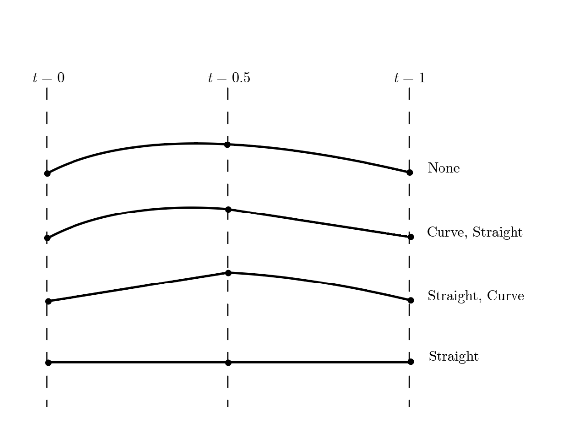
We initialize all experiments with the EDM model⁸. We then generate the Reflow triples using the EDM model for all timesteps. Now we split the generation time into two parts. At train time, we can run the Reflow operation to straighten or not straighten the first half, and straighten or not straighten the second half. So we can either straighten or not straighten for each of the halves, giving us $4$ different settings of how we train our models.

Furthermore, at test time, we experiment with using more or less steps for the first half and the second half. Intuitively, if it is okay to assume a straight path in each of these halfs, using less steps should not diminish sample quality. This leads to $4$ different settings of how we allocate our steps to each half of the generation process. Concretely, we either use $1$ or $9$ steps for the first or second half of the generation process.

Overall, we combine these two parts to achieve $4\times 4 = 16$ settings for our experiments. We choose MNIST for our dataset. We refer to the first half of the generation process (where we start from noise) as the left side and the second half as the right side. From here on, our models are referred to as

• None: no straightening applied.
• Left: straightening on the left side.
• Right: Straightening on the right side.
• Both: Straightening on both sides.

---

Results

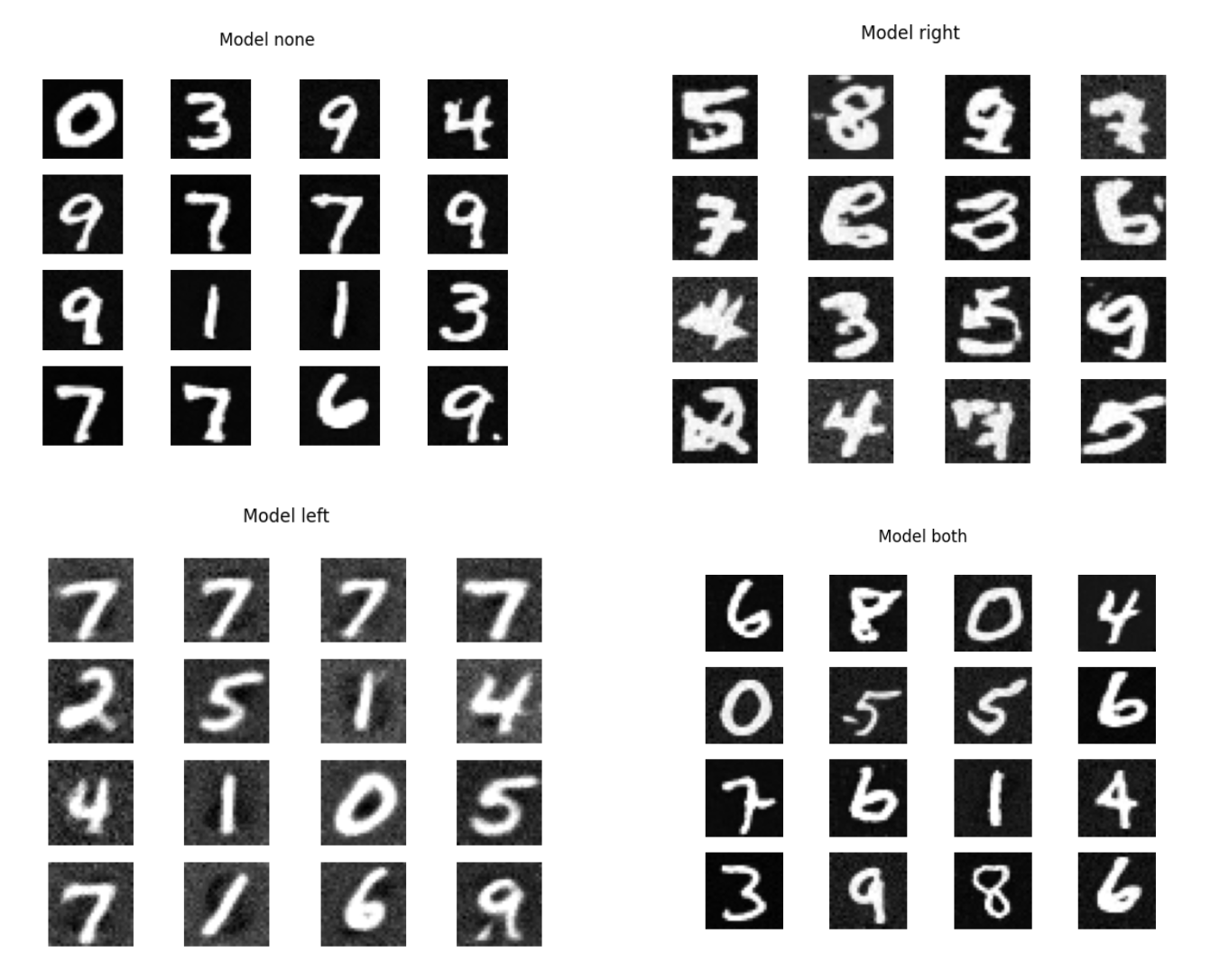
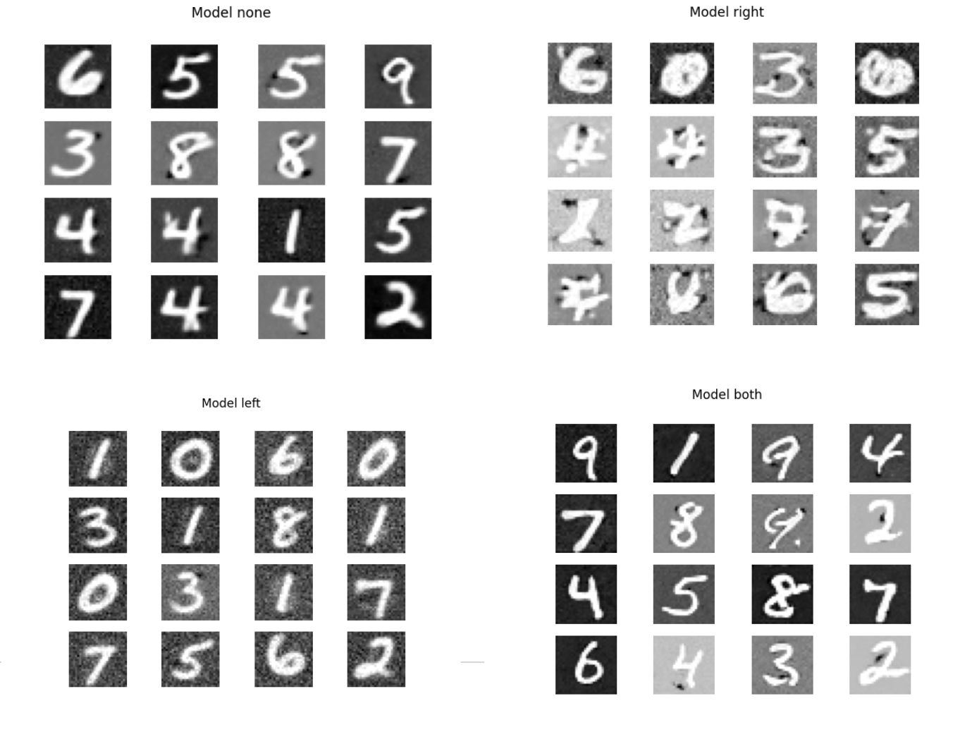
We observe that straightening in the early time range where the data is mostly noise is better than straightening in the later time range. This aligns with our hypothesis that it is okay to straighten out the lower frequency part of the generation process. In addition, allocating more steps in the earlier time range gives comparable performance to allocating more steps in the earlier time range, given that we allocate the same number of steps to the second time range. This again aligns with our hypothesis that it is okay to allocate less computation time to the lower frequency portion of the image generation process.

Future Directions

The results for reflowing on only half of the trajectory was noticeably degraded from reflowing on both halves of the trajectory even though only half of the trajectory was finetuned. This indicates that there is degradation of the predictions on the second half of the model. Perhaps a way to remedy this would be continue training on the half we wish to keep constant with the ground truth coming from the original pre-trained flow matching model.

Further tricks that could be done to improve the performance of ``half-straightening'' can be found in Lee et. al.⁷. Different loss functions (such as LPIPS or Pseudo-huber) could be incorporated, different timestep sampling procedures could be used, or even original MNIST data could be added to prevent degradation of samples. In all, our experiments show proof of intuition on where you can mess with the trajectory, but may not be a very practical method of generative modeling until more engineering is done on it.

Code for experiments can be found here: https://github.com/12tqian/6.s978-final-project

---

Footnotes

1. Ruiqi Gao et al. “Diffusion Meets Flow Matching: Two Sides of the Same Coin”. In: 2024. url: https://diffusionflow.github.io/. ↩ ↩²

2. At least, when the latent distribution is a Gaussian. ↩

3. Jiaming Song, Chenlin Meng, and Stefano Ermon. “Denoising diffusion implicit models”. In: arXiv preprint arXiv:2010.02502 (2020) ↩

4. Yilun Xu et al. Restart Sampling for Improving Generative Processes. 2023. arXiv: 2306.14878 [cs.LG]. url: https://arxiv.org/abs/2306.14878. ↩

5. Qiang Liu. “Rectified flow: A marginal preserving approach to optimal transport”. In: arXiv preprint arXiv:2209.14577 (2022). ↩ ↩²

6. Xingchao Liu et al. “InstaFlow: One step is enough for high-quality diffusion-based text-to-image gen- eration”. In: arXiv preprint arXiv:2309.06380 (2023). ↩

7. Sangyun Lee, Zinan Lin, and Giulia Fanti. Improving the Training of Rectified Flows. 2024. arXiv: 2405.20320 [cs.CV]. url: https://arxiv.org/abs/2405.20320. ↩ ↩²

8. Tero Karras et al. “Elucidating the design space of diffusion-based generative models”. In: arXiv preprint arXiv:2206.00364 (2022). ↩